Small Isolation Chamber

Open Source Instruments Inc. has moved from 397 Moody St, Waltham, MA, to 5 Pratt Ave, Waltham, MA. Our new office is a 180-m² basement with a concrete floor and plenty of half-windows.


Figure: New OSI Location: 5 Pratt Ave, Waltham, MA.

On Moody St, interference power picked up by a Damped Loop Antenna (A3015C) in the 925-928 MHz band was up to −58 dBm (1.6 nW). Here on Pratt Ave, the same 925-928 MHz power peaks at −45 dBm (32 nW). On a work bench, reception from a subcutaneous transmitter only at ranges less than 10 cm. Interference power in our new office is four times greater than in any other place we have measured (London, Oxford, Edinburgh, Guildford, Waltham, Boston). Our new location is a fine place to test the efficacy of radio-frequency isolation chambers.

We set up a small isolation chamber. It consists of six AN-77 absorbers, gray sides inwards, standing on the concrete floor. We wrap an outer layer of resistive sheet around the absorbers. We put a cover of the same resistive sheet on top. We assume the floor is a perfect absorber, because we are in a basement.

Figure: Small Isolation Chamber on Concrete Floor.

We set up our A3008C spectrometer and measure 925-928 MHz interference power for one minute with the pick-up antenna on the corner of our work bench, on the floor out in the open, in the center of our isolation chamber, and in the corner of our isolation chamber.


Figure: Interference Power in Separate Minutes and in Various Locations.

The peak interference power outside the enclosure is −45 dBm. Inside the chamber, the power never rises above −68 dBm (160 pW). The chamber appears to provide 23 dB of isolation. We place a Subcutaneous Transmitter (A3019D) inside the chamber 50 cm from each of two antennas connected to an Octal Data Receiver (A3027C). Over the course of one minute we obtain 100.0% reception. We remove the enclosure lid and reception drops to 29%.

Command Transmission Noise

We turn on two Subcutaneous Transmitters (A3019). One has 150-mm leads and the other has 45-mm leads. We place the tips of the leads in water, so that they are connected by an impedance of order 100 kΩ. This connection reduces the amount of mains hum the transmitters pick up, allowing us to see other sources of noise. We turn on our Command Transmitter (A3023CT), which emits pulses of 146-MHz radio-frequency power to stimulate Implantable Lamps (A3024). We place the command antenna 70 cm from our two subcutaneous transmitters, and instruct the command transmitter to emit 10-ms pulses at 10 Hz. We see the following response from the subcutaneous transmitters.


Figure: Command Transmission Noise. Two A3019 subcutaneous transmitters responding to pulses of 146-MHz command pulses. Vertical range is 27 mV, horizontal range is 500 ms. Pulses are 10 ms at 10 Hz. Pink trace: 150-mm leads. Orange trace: 45-mm leads.
If we remove the leads from an A3019, we see no response to the command transmission. We record with a two-channel Subcutaneous Transmitter (A3028D) and observe the same pulses on both channels. We suspect that the leads pick up 146-MHz power, which penetrates the transmitter circuit and is somewhere demodulated by a non-linear element in the amplifier. The demodulated signal is added to the input, resulting in pulses. We record the following trace from an A3019 without encapsulation and equipped with 150-mm wire leads.


Figure: More Command Transmission Noise. One un-encapsulated A3019 responding to pulses of 146-MHz command pulses. Vertical range is 27 mV, horizontal range is 500 ms. Pulses are 10 ms at 10 Hz.
We add a 100-kΩ resistor in series with each lead, and a 10-pF capacitor at the far side of the resistors. Thus the resistors form a high-pass filter with cut-off frequency 80 kHz. At 146 MHz, the filter attenuates by a factor of two thousand in amplitude. A 20-mV pulse of command transmission should be reduced to 1μV. With the filter installed, we recording the following trace from the subcutaneous transmitter with the same command pulses.


Figure: Eliminated Command Transmission Noise. One un-encapsulated A3019 equipped with 80-kHz low-pass filter showing no response to pulses of 146-MHz command pulses. Vertical range is 27 mV, horizontal range is 500 ms. Pulses are 10 ms at 10 Hz.
The 10-pF capacitor of the filter appears in parallel with the 10-MΩ input impedance of the subcutaneous transmitter's EEG amplifier, making a low-pass filter with cut-off frequency 1.6 kHz, which is above the 1.3-kHz bandwidth we would obtain from an A3019 running at 4096 SPS. The two 100-kΩ resistors form a divider with the 10-MΩ input impedance, which reduces the EEG signal amplitude by 2%, which is insignificant. We claim this filter will have no effect upon the detection of EEG, and yet eliminates the command transmission noise.

Taper Power Measurement

We have three ways to measure the power emitted by a glass taper. For all methods, we mask the LED with black tape and we use our SD445 photodiode. The photodiode measures 10 mm × 10 mm. With no reverse bias, this photodiode has sensitivity 0.18 mA/mW at 460 nm (see LED Efficiency). In the first method, we measure the light intensity emitted in an array of directions and integrate over a hemisphere to obtain total emitted power. In the second method, we place our photodiode in five locations to make a virtual cube of photodiode 10 mm on each side, centered on the taper. We add the photocurrents together and so obtain an estimate of total power. In the third method, we hold the photodiode as shown below.


Figure: Single-Location Measurement of Taper Power Output.
The transparent plastic surface of the photodiode reflects light with angle of incidence greater than 80°. The above arrangement results in the photodiode receiving light emitted by the taper within a ±80° wedge in the horizontal plane. To obtain total power emitted, we multiply the photocurrent by 360°/160° = 9/4 and divide by the sensitivity 0.18 mA/mW.

Of our three methods, the first is the most time-consuming and prone to error. The second is prone to error due to incorrect placement of the photodiode. The third is the easiest. We measured the power output of A3024HFB No2.9 with Method Two and obtained 10.8 mW at 30 mA forward current. We applied Method Three and again obtained 10.8 mW. From now on we will use Method Three and assume it is accurate to ±10%. We will refer to Method Three as the angled photodiode method. We use the angled photodiode method to measure total power output versus forward LED current for A3024HFB No2.9, and obtain the following plot.


Figure: Taper 2.9 Output Power versus LED Forward Current.
We see that the taper emits roughly 11 mW at 30 mA, 18 mW at 50 mA, and 22 mW at 70 mA. When the forward current is above 50 mA, however, the output power drops during the seconds after we apply the current. Thirty seconds after we apply 80 mA, the power has dropped by 10%. This drop is due to self-heating of the LED.

New Head Fixture

We have a new head fixture printed circuit board. It provides a notch for the guide cannula, rather than a hole. There is a two-way plug for delivering power during assembly, and two miniature sockets for pins during implantation. We mount ten C460EZ500 LEDs in QFN-8 packages into ten such circuit boards and measure their power output at various forward currents.


Figure: We give diameter of fiber we later glued to the LED and the coupling efficiency. The coupling efficiency is the fraction of light emitted at 30 mA that emerges from the fiber tip.

In series with the LED is a surface-mount resistor that allows us to set the LED forward current once we know the length of the power supply leads. We expect the leads to be 50 mm long in mice and 150 mm long in rats. The resistance of our stretched helical 100-μm wire leads is 10 Ω per 50 mm. The power supply is 5 V and the LED forward voltage is 3.2±0.1 V for currents of order 50 mA. With a 0-Ω resistor and 150 mm leads we will get 32 mA. With a 7-Ω resistor and 50-mm leads we will get 70 mA, assuming the battery can supply the required current to its boost regulator.

We make an 8-mm long fiber of higher-index glass. The fiber has a 2-mm taper at one end a flat on the other. Its diameter is 440 μm. We its base onto the center of the LED. We squash down the bond wire, but there remains a gap of roughly 100 μm between the fiber base and the LED surface. Our calculated coupling efficiency for a fiber with outer diameter 440-μm and numerical aperture 0.86 is 47%. We expect to lose 2% of this light in the yellow glass of the fiber, which will reduce our coupling efficiency to 46%. Our calculation assumes, however, that the LED and fiber surfaces are touching.


Figure: Higher-Index Taper Glued to Blue LED. Assembly number A3024HFB, serial number 2.10.

We mask the base of the fiber with tape and pass 30 mA through the LED. We measure the photocurrent in our 10 mm × 10 mm photodiode at range 20 mm for the fiber tip. We vary the angle, θ, between the axis of the fiber and the line joining the tip to the center of the photodiode. We orient the photodiode so its surface is always perpendicular to this line. For θ = 90° we go around the fiber in a horizontal plane in 45° steps. The light intensity varies from 50-110 μW/cm², with an average of 80 μW/cm². We move the photodiode in a vertical plane and vary θ from 90° to −90°. We obtain the following plot of intensity versus angle.


Figure: Intensity versus Off-Axis Angle for Fiber Tip. The fiber base is masked with black tape. We move our 1 cm² photodiode around in a vertical plane at range 2 cm. Assembly number A3024HFB, serial number 2.10.

By integrating this curve for the hemisphere above the taper, we obtain a crude estimate of 9 mW for the total emitted power. To obtain a better estimate, we place our 1 cm² photodiode in five positions on four sides and above the tip of the fiber, at range 5 mm, so as to make a cube that receives all emitted power. We add the photocurrents thus obtained, after subtracting for background light, and arrive at a total of 1.76 mA, which suggests a total output power of 9.8 mW at 30 mA forward current. Given that this LED emitted 26.7 mW at 30 mA, our coupling efficiency to the tip is 37%. We increase the LED current to 50 mW and optical power output increases by 45% to approximately 14.3 mW. For the first time, we have a taper that emits roughly 10 mW with forward current 30 mA. If we increase the LED current to 70 mA, which will be possible with a rat-sized lithium-ion battery, this fiber tip will emit 19 mW. This fiber's coupling efficiency is 37%, compared to a theoretical maximum of 46%.

To complete the head fixture, we need a 9-mm silica guide cannula. Our existing guides are 7-mm long. Our plan is to glue the tip of the guid to the base of the taper, and measuring with the existing taper, the guide cannula length below the plastic thread must be 9 mm.

UPDATE: [24-DEC-13] In No2.2, we use the offset placement of the fiber shown here, which allows us to press the fiber base onto the surface of the LED. We get 5.7 mW for 30 mA, or 22% coupling efficiency.

UPDATE: [23-JAN-14] By squeezing the fiber clamp with our fingers, we force the fiber base closer to the LED surface. This appears to increase our coupling efficiency from 37% to 38%.

UPDATE: [24-JAN-14] We take out head fixture A3024HFB No2.6 and measure its power output with 30 mA. We mask the LED with aluminum foil. With angled photodiode we get 10.4 mW total power output. With the fiber perpendicular to the photodiode and the tip touching the photodiode, we get 1.3 mA of photocurrent, or 7.3 mW incident light. Given that the photodiode extends for 5 mm from the tip, and the light emission takes place along a 1-mm length, everything emitted within ±84° of the fiber axis is incident upon the photodiode. The missing 3 mW must be emitted at an angle greater than ±84°.

Manufacturing Precision Tapers

As discussed in our last post, we've equipped our tapering machine with a custom-made electric heating element. This gives us precise temperature control, allowing us to soften the glass without melting it. The electric heater has the added benefit of not introducing a stream of air flow which may otherwise distort the taper (as is the case with torch flames). It also has the benefit of not removing the cladding layer, as is the case with laser machines. Our stretching machine uses two translating stages driven by stepping motors. We program them with machine code (via a LWDAQ interface), allowing an infinite range of stretching algorithms to choose from.

Our goal is to be able to consistently manufacture a specified taper profile. Good tapers must have the following properties:

- Specified profile; Typically, the walls of the taper are linear (flat) or slightly convex. The length of the tapered region is specified.
- Axial symmetry
- Sharp tip

Additionally, the manufacturing process must produce repeatable results so that tapers appear identical to one another. Through much experimentation, we've discovered guiding principles for designing heaters and stretching algorithms that produce high quality tapers.

Our latest effort has been to produce medium length tapers out of our 410-μm high-index fiber. We developed a stretching algorithm that self terminates the taper. This leaves a sharp point and improves consistency by eliminating the need for a human to trim the taper to length. The result is a 2.7mm taper with high axial symmetry. While viewing the taper through a jeweler's loupe and rotating it, any deviation from axial symmetry is difficult or impossible to discern. Three such tapers were made consecutively and are shown in the image below.


Figure: Three 2.7mm tapers made of 410μm High-index fiber. The ruler's tick marks are 0.5mm apart.

We will continue to experiment with methods to control the manufacturing process for even better consistency. These include improving the consistency of our heater's power source and consideration of the slight variations in the diameter of the fiber as supplied by its manufacturer. We will also experiment with algorithms that produce shorter or longer tapers as required.

Higher-Index Taper

In one of our earliest posts, we described how an electric heating element was unable to heat silica-silical fiber to its 1100°C softening point. Our high-index fiber and our higher-index fiber soften at around 430°C. We equip our motor-driven tapering machine with a coil of nichrome wire, potted in high-temperature cement and produce the taper shown below.


Figure: Taper in 410-μm Higher-Index Fiber. Blue 460-nm light. Taper is 2.0 mm long.

The taper shown above is at the top of a 40-mm shaft of higher-index fiber, polished at the base. Its diameter is 410 μm. We lower the base onto a C460EZ500 blue LED die. This particular LED has output power 27 mW (4.85 mA photocurrent through unbiased photodiode) for forward current 30 mA. Because we were in a hurry, we fastened the fiber to the LED with five-minute epoxy. We bake it in our oven at 60°C and within twenty minutes, the epoxy is fully cured.

We drive 30 mA through the LED. We press our 10 × 10 mm² photodiode against the side of the fiber, so that the axis of the fiber is a millimeter from the photodiode window. We expect light emitted by the taper more than 20° from the fiber axis, and in a ±80° slice in the radial direction, to enter the photodiode. We see 3.7 mW (0.67 mW photocurrent). We hold the photodiode 15 mm from the top of the taper, and perpendicular to the fiber axis. We now receive most of the light within ±20° of the axis. We see 1.1 mW (0.2 mA photocurrent). Multiplying the first measurement by 2*9/8 and adding the second, we arrive at 9.4 mW total emission from the taper. Assuming 2.2% loss per 10 mm, the power entering the base of the fiber should be 10.3 mW, which is 38% of 27 mW.

We produced four such tapers from two lengths of higher-index fiber polished at both ends. The one we show above is the shortest. We can make them in the same machine with 6 mm of fiber followed by 2 mm of taper. Such a fiber would emit around 10 mW from its tip for 30 mA of LED current.

Yellow Glass

Yesterday we were mystified when our coupling efficiency dropped from 39% to 21% when we applied glue to the base of a 146-mm higher-index fiber. Today the epoxy is cured. The fiber is attached firmly. There are only a few small bubbles in the glue, towards the surface. We apply 30 mA to the LED. When the glue was curing yesterday, we obtained only 5.3 mW at the top end of the fiber. Today we obtain 8.2 mW. Yesterday the total power output of the LED at 30 mA was 25.7 mW. Our capture efficiency appears to be 32% now the glue has cured, but was only 21% while it was liquid.

Most of our 146-mm fiber is in air. The bottom 4 mm are covered with glue of refractive index 1.5 and a 3-mm section is clamped in steel. It may be that some light is propagating up the fiber in the cladding by total internal reflection at the cladding-air boundary. We apply clear epoxy to 30 mm of the fiber, near the top. The power at the tip remains 8.2 mW. We conclude that the 4-mm coating of epoxy at the base is sufficient to cause the loss of all light except that which is captured by the core.

We cut back the 146-mm fiber to 30 mm and polish the tip. We apply 30 mA and obtain 10.6 mW at the new tip. The fiber and LED are shown below. The conical angle of the emission from the fiber tip is around ±60°, which is consistent with a numerical aperture of 0.86.



Figure: A 30-mm Higher-Index Fiber. Click on image for higher resolution. The base is glued to a C460EZ500. The tip is polished.

The T5 glass used by Fiberoptics Technology is a proprietary glass with index 1.72. The manufacturer tells us the glass is "very yellow", which we take to mean that it absorbs blue light. A similar glass with index 1.72 made by Schott, P-SF69, has transmission over 10 mm of 98.5% at 460 nm. Suppose the T5 glass has transmission η after 10 mm, and the power coupled into our fiber at the base is P, then Pη^3.0 = 10.6 mW and Pη^14.6 = 8.2 mW. From this we conclude that P = 11.3 mW and η = 97.8%.

With 11.3 mW out of 25.7 mW being coupled into the core of our fiber, our coupling efficiency is 44%. Our calculated coupling efficiency for this arrangement is only 38%. It may be that the LED is producing more power today than yesterday. If it is producing 28 mW, which is what we are hoping for from these LEDs, then the coupling efficiency is closer to 40%.

Yesterday, we were mystified because we assumed our fiber in air was not able to transport light in its cladding, because of dirt on its surface, and because of the metal-glass contact in the fiber clamp. And we had forgotten about the absorption of blue light by this high-index glass. Furthermore, there appears to be some problem with the coupling when the glue is liquid, and this we still do not understand.

We have a fiber that produces 10.6 mW at its tip with 30 mA LED current. If we taper the fiber to a total length of 8 mm, which is our intention for the head fixtures, we expect to get 11 mW out of the taper. If we increase the LED current to 50 mW by using shorter steel leads, the power at the taper should increase to around 18 mW.

Gluing Loss

We take a 150-mm section of our higher-index fiber (NA = 0.86) and polish it at both ends. The diameter of this section is 410 μm.. We lower one end onto a C460EZ500 blue LED die. According to our diameter and location simulation, the best coupling of light from the LED to a 410-μm fiber occurs when the fiber is roughly 40 μm offset from the center of the die, in the direction opposite to the bond pad. We calculate that 58% of the light emitted by the LED will be incident upon the fiber base.

In practice, however, we find we cannot lower the fiber into this optimal position because the wire bond on the bond pad is around 100 μm high. We tried raising the fiber above the wire bond, but we obtained the greatest coupling efficiency with the fiber placed flat on the surface of the LED as close to the center as we can get it. The result is shown below.


Figure: Offset Fiber. This 410-μm diameter fiber is roughly 120 μm from the center of the EZ500.

With the fiber 120 μm from the center, our incidence calculation suggests we will get 52% of the LED light incident upon the base of the fiber. With NA = 0.86, we expect 74% of the light incident upon the base of the fiber to emerge at the other end, for an expected total capture efficiency of 38%.

We run 30 mA of current through the LED. The power emitted by the far end of the fiber is 9.8 mW (photocurrent 1.77 mA and sensitivity 0.18 mA/mW). We remove the fiber and measure 25.2 mW total power output (photocurrent 4.53 mA). Our coupling efficiency is 39%. We re-position the fiber several times. We obtain 38% or 38% coupling efficiency each time.

With the fiber in place, we inject E-30CL clear optical epoxy (RI = 1.5) into the LED package. The epoxy flows around the fiber and LED. The result is shown below, with a few milliamps of current in the LED.


Figure: Offset Fiber with Clear Glue.

As soon as the glue has surrounded the LED, the power at the fiber tip drops from 9.8 mW to 5.3 mW (photocurrent 0.95 mA). We raise up the base of the fiber and remove it from the glue blob and measure the total LED output to be 25.7 mW (photocurrent 4.62 mA). We replace the fiber and place it in its previous position. Once again we obtain 5.3 mW at the fiber tip. Our coupling efficiency has dropped from 39% to 21% with the application of glue.

Right now we have no explanation for this dramatic drop in coupling efficiency with the application of glue. So far as we understand, the a thin layer of transparent material between the fiber and LED will not stop light entering the fiber. Nor will glue on the outside of the fiber reduce its numerical aperture below 0.86. Nevertheless, the effect is real and repeatable. We have observed it many times, today being merely the most detailed observation of the effect to date.

Isolation Chamber for IVC Rack

When we apply the principles presented in Radio-Frequency Isolation Chamber, we arrive at the following solution for enclosing a large IVC (Individually Ventilated Cage) rack, such as the AERO80 from Tecniplast.


Figure: Proposed Radio-Frequency Isolation Chamber for a Large IVC Rack.
The chamber consists of absorber back and side walls, reflecting front wall and base mat, and open ceiling. Our sketch does not show the ventilation ducts entering and leaving the rack, but these can pass out above and below, or to the rear of, the side walls. The rear wall is 1.83 m square, made of 9 AN-77 absorbers. The gray side of these absorbers faces the cages in the rack. The black side is glued to an aluminum backing, which faces outward. The side walls are of the same construction, but made of 3 AN-77 absorbers each. In front of the rack is a curtain of transparent, conducting steel mesh. Below is a rubber mat that conceals a sheet of conducting fabric.

Radio waves approaching the isolation chamber are reflected away unless they pass through a gap or the ceiling. Such waves will pass through the rack once. If they arrive at an absorber wall, the chance of them being absorbed rather than reflected is 98.2%. If they hit the curtain or the mat, they will certainly be reflected, and so pass through the chamber a second time. If they reach the ceiling, they will exit the chamber. Such a chamber should reflect away 90% of incident interference. Some of the interference entering the chamber will pass through its volume twice because of the front and bottom reflectors, so interference power inside will be of order 15% the power outside. This 85% isolation is sufficient to guarantee 70% reception from an implanted transmitter at range 30 cm in the presence of −48 dBm interference, which is the strongest we have observed.

We arrange the eight independent antennas of Data Receiver (A3027B) on the shelves of the IVC rack. The sketch below shows how we might arrange these antennas to record from eight animal cages.


Figure: Proposed Arrangement of Antennas in an IVC Rack.
If we have a = b = 30 cm, and we consider the top-right cage, with an implanted transmitter on the far-right of the cage, we see that our arrangement provides two antennas at 30 cm, one at 42 cm and another five at greater ranges. We note that, because of the reflecting curtain at the front, there are two paths for radio waves to reach more distant antenna from our top-right transmitter. If we assume 70% reception for antennas at 30 cm, 50% from the antenna at 42 cm, and 20% from antennas up to 120 cm, and we further assume independence of message loss, we expect combined reception to be 98.5%.

We propose that ION perform the detailed design and construction of the rear and side absorber walls and the curtain rail. The walls should support the absorbers a few inches above the ground, and we should be able to remove each wall independently for comparative tests. The curtain rail likewise we should be able to remove with the entire curtain attached. We further propose that ION will select a rubber mat suitable for supporting the rack above the base reflector. At OSI, meanwhile, we will sew together the steel mesh curtain and cut the base reflector. We will prepare an A3027B Data Receiver and design a new loop antenna that fits easily between cages. We will provide transmitters to implant if necessary, so that we can test reception from within live animals.

UPDATE: [28-FEB-14] We make a curtain 2.0 m wide and 2.2 m high with curtain rings for the chamber test at ION. We hang the curtain in our office. We lay down a mat of copper teffeta fabric. We make a 1.2 m × 1.2 m absorber back wall and two 1.2 m × 0.6 m side walls. We suspend a piece of resistive sheet above the isolation chamber thus created. The result is shown below.



Figure: Isolation Chamber with Front Curtain.

We place three antennas on a table inside the chamber and three transmitters, which we move around to different places on the table. Reception without the chamber is 0-100% because of intermittent −58 dB ambient interference at 926 MHz. With the chamber as shown, we get reception 95-100%. When we move aside the curtain, reception drops to 70-100%. Peak interference power in the closed chamber is around −64 dB.

Radio-Frequency Isolation Chamber

A Faraday Cage provides isolation by reflecting incoming RF (radio-frequency) waves. We could instead provide isolation by absorbing incoming waves. The AN-77 is a 61-cm square of conducting foam that absorbs 90% of incident 900-MHz radio waves when it is free-standing without a conducting backing. We set up the following chamber on our office floor.


Figure: Coffin-Like Absorbing Enclosure. Floor is reflecting sheet, walls are AN-77 absorbers.
The purpose of any chamber we might build around our SCT system is to promote reliable reception. The chamber can do this in two ways. One is to attenuate external interference. Another is to increase the power we receive from our transmitters. Our new Data Receiver (A3027) provides eight independent antenna inputs. Each has its own amplifier, demodulator, and message detector circuit. With eight antennas, we need only one to pick up a transmitter message. An isolation chamber with one or two reflecting walls can make it more likely that a message will be received by an antenna 100 cm away.

In the coffin-like enclosure shown above, we see three antennas on the floor. These are each independent and connected to our prototype A3027. They are separated by 30 cm, which is enough for a rat cage. We hold an A3019D transmitter in our hand, with the antenna protruding into air, and move and rotate it at random in the 30-cm cube between the left and center antenna. We obtain 100.00% reception over one minute. That is to say: we do not lose a single message. If we disconnect the right-most antenna, reception drops to 98.2%, and if we disconnect the left-hand antenna as well, reception drops to 96.6%. We perform the same measurements with the entire transmitter and antenna enclosed in our hand, so the antenna is enclosed in human tissue at least 2 cm deep. We connect all three antennas. We obtain 99.3% reception. We remove the enclosure and repeat our measurement with only the center antenna connected, and the transmitter in our fist. We obtain 38% reception.

Interference power in our office is −48 dBm, which is as great as we have seen in any laboratory. Reception with one antenna at ranges up to 30 cm is only 38% when we mimic implantation by holding the transmitter in our fist. With three antennas inside our coffin-like absorbing enclosure, however, reception rises to 99.3%.

The dramatic improvement in reception is provided by the slight attenuation of external interference provided by the absorbing walls of the coffin. But it is also provided by the reflection of radio-waves towards the more distant antenna by the floor of the enclosure. Within the chamber, we are more likely to pick up signals with the distant antenna than outside.

Thus we propose to place a wall of absorbers behind and to either side of an IVC rack, a curtain of conducting mesh fabric in front, and a mat of conducting fabric below. These precautions, when combined with eight independent receiving antennas, may give us reliable reception inside the rack.

Now suppose we have two such racks in one room. Our absorbing enclosure will not guarantee that the antennas in one rack will not pick up signals from the other rack. Reception from the neighboring rack may be poor and rare, but it cannot be stopped entirely. Thus we must add one more feature to our SCT system. We propose that new transmitters broadcast a set number between 1 and 15 after their existing message bits. Meanwhile, we will be able to configure our A3027 data receivers so that they reject messages from all but one set number. Thus we can operate transmitters with set number 1 in an IVC rack next to transmitters with set number 2. The transmission of the set number will come at a slight cost in current consumption: battery life will drop by roughly 10%.

The scheme we have described has the advantage of being far more practical than the original sealed and reflecting faraday enclosure. We merely hang walls of absorbers around the back and sides of the rack. We have a curtain that can be pulled aside from the cages in front. We do not have to seal any gaps. Our multiple antennas and the transmitter set numbers provide reliable reception at the same time as stopping cross-talk between adjacent SCT systems. Our hope is to test this scheme at ION at the end of October.

Failure of the Faraday Canopy

Our FE2B Faraday enclosure provides a minimum of 20 dB (99%) rejection of interference power. As we described earlier, we hoped to duplicate this performance on a larger scale, so as to enclose an entire IVC (Individually Ventilated Cage) rack. The photograph below shows our faraday canopy with three towers of AN-77 absorbers in a triangle. Each AN-77 absorber is 61 cm square.


Figure: Triangle of Absorber Walls in the Faraday Canopy. Kirsten is standing still so as to allow us to obtain a stable interference measurement with the antenna resting upon the stool.
With no absorbers in the canopy, we usually obtained 10 dB isolation. With six AN-77 absorbers standing on the floor, we sometimes obtained 20 dB isolation, but often as little as 6 dB. With nine AN-77 absorbers in a wall 1.8-m square, we usually obtained 20 dB isolation, but sometimes as little as 6 dB. In one experiment, we observed the isolation to changed from 7 dB to 20 dB as the experimenter inside the enclosure changed where she was standing. (You will find a complete account of our experiments here.)

If we are to enclose an IVC rack, we must accommodate the two ventilation pipes. Catherine tried running the ventilation through steel mesh fabric, in the hope that we could simply pass the air through the sealed enclosure, but the result was dirt building up in the mesh, which degraded the performance of the ventilation. Thus we would have to insert two breaks in the enclosure of around 10 cm diameter each. This diameter is one third of our 900-MHz radio-frequency data wavelength, and so would allow interference to enter the cage, and once inside, the interference would reflect off the canopy walls until it struck an absorber. A sock of reflecting mesh around the ventilation pipe will not stop the penetration of interference, because once inside the sock, the radio waves will continue bouncing along its length until they enter the enclosure.

Even if we could improve the isolation of such an enclosure to 20 dB in the presence of ventilation holes, there remain many practical difficulties in moving the IVC rack into and out of the enclosure, and in supporting a sealed enclosure around the rack. Thus we have abandoned our plan to make a faraday canopy for the IVC. But we do have an alternative, and we will describe this alternative in our next post.

(NOTE: Our continuing work on radio-frequency isolation for IVC racks is funded by a budget separate from our ISL development budget, but we present the work here for want of a better venue, and because it is relevant to the ISL implementation.)

UPDATE: [01-JAN-14] We suspect that the poor performance of our faraday canopy is due to the canopy itself acting as a resonator in combination with the shield of our pick-up antenna cable or with the antenna itself. Any break in the canopy, such as an imperfect seam, can turn the canopy from an isolation chamber into a resonant cavity, as described here. Our cable sock will act as such a break, and cables passing through the sock can act as one half of a dipole antenna with the canopy, picking up energy incident upon the outside of the canopy. Solving these problems would be impractical for a canopy used in animal experiments, in which the experimenter should be able to enter and leave easily, and through which we must be able to pass ventilation pipes.

UPDATE: [28-FEB-14] We set up the faraday canopy in our new office. Ambient 902-930 MHz interference peaks at −43 dBm on our work bench. It enters via the roof and windows only, because we are in a basement. We place three antennas inside the cage, one on the floor and two on a box. We tape the shields of all three cables to the copper fabric floor of the canopy. Interference peaks at −61 dB, −52 dB, and −64 dB on the floor, box, and box.

Higher-Index Fiber

We receive from Fiberoptics Technoligy a new batch of fiber. As with our High Index Fiber, the core occupies 83% of the cross-section and the cladding the remaining 17%. This time, the core is made of a proprietary glass of refractive index 1.72, which they call TD5. The cladding is Schott 8250. The core numerical aperture is 0.86.

The fiber is divided into 178 sections, each 9 m long, so that the total length of fiber is around 1600 m. We took a 10-cm sample from each 9-m section and measured its diameter. Of these, 165 had diameter 390-440 μm, and 13 had diameter 130-310 μm. We set aside the thinner fibers and consider the 165 larger fibers. The histogram below shows the distribution of their diameters.


Figure: Distribution of Section Diameter

We were hoping for an average diameter of 440 μm and a range of 400-480 μm. What we have is an average diameter of 411 μm with range 390-440 μm, which is similar to the distribution of our previous high-index fiber.

From the 1600 m of fiber we have 100 m with diameter 430 μm or higher. We need 50 mm to make one 8-mm fiber taper, so we have enough fiber in stock to make two thousand fiber tapers of base diameter 430 μm. According to our calculations, the 430 μm diameter should capture and transport 64% of the light emitted by an EZ500 LED. With 30 mA of LED current and 28 mW of blue light emitted, we are hoping to see 18 mW at the fiber tip.

UPDATE: [28-JUN-13] We find a piece of TD5 fiber with diameter 450 μm. We polish both ends of a 80-mm length. We cover 20 mm of the fiber with nail polish. We run 30 mA through an EZ500 460-nm blue LED and obtain 31 mW emitted power. We lower the fiber onto the LED and obtain 16 mW at the fiber tip, which is 50% capture efficiency, and consistent with our earlier calculations for a fiber of numerical aperture 1.72 and diameter 450 μm.

Diameter Variation

We have of order 300 m of optical fiber with numerical aperture 0.66 (core index 1.63, cladding 1.49). When we first received the fiber, we measured its diameter in one place and obtained a value 390 μm. Since then, we have assumed all fibers we cut from our 300-m batch are 390 μm in diameter. Today we cut 225 sections each roughly 30 cm long from our 300-m batch. We measured the diameter of each section with a micrometer. Our resolution in measuring diameter is 3 μm with our micrometer. We obtain the following histogram.


Figure: Distribution of Diameter Among Samples.
The nominal diameter of the fiber, as supplied by Fiberoptics Technology, was 0.016", or 406 μm. We find the average diameter to be 405 μm, with standard deviation 12 μm. The minimum diameter is 370 μm and the maximum is 440 μm. We measure diameter along the length of a selection of fibers and obtain the following plots. The most rapid change in diameter we observe along a fiber section is 30 μm in 100 mm. Along an 8-mm ISL fiber, we would see no more than a 0.6% change, which is insignificant for our purposes.


Figure: Changes in Diameter With Position.

The following graph uses shows how we expect the coupling efficiency of a fiber to increase with diameter, using the calculation we presented in Diameter and Location, and assuming optimal positioning of the fiber on a blue EZ500 die. We assume that the fiber always has 87% of its area occupied by the core, and we consider only the light entering and captured by the core.


Figure: Calculated Coupling Efficiency versus Outer Diameter of Fiber. We show the light incident upon the core of the fiber base as a function of outer diameter of the base, and we show the light fraction of light carried to the far end for NA = 0.66 and NA = 0.86.

We observed 27% and 30% coupling efficiency with sections of our NA = 0.66 fiber. Until now, we assumed the fiber diameter was uniformly 390 μm, and so we were puzzled with these high coupling efficiencies. But we now see that a diameter of 420 μm would give us close to 27%, and 440 μm would give close to 30%.

We plan to order NA = 0.86 fiber (core index 1.72, cladding 1.49) from Fiberoptics Technology. Variation in diameter as we observe in our NA = 0.66 batch would serve us well, because we would have a range of diameters to choose from. A nominal diameter 440 μm (0.0173") with tolerance ±35 μm (0.0014") should produce a useful batch.

Diameter and Location

We obtain the following picture of 460-nm EZ500 flashing with 80-mA forward current for a few microseconds. We obtain the photograph with a Camera Head (A2075B) and two neutral density filters. Only 0.1% of the light emitted by the LED passes through the filters.


Figure: Intensity of Light At Surface of Blue EZ500

We extract the pixel intensities from this image and find that the intensity at the center is double the intensity near the edges. We write a program that calculates how much light will be incident upon the base of a fiber pressed against the LED surface, as a function of the fiber diameter and its offset from the center of the LED square.


Table: Calculated Fraction of EZ500 Light Incident Upon Fiber Base. We assume the core is 83% of the cross-section, or 91% of the diameter. Also shown are the fraction of light that will be coupled to the core for various fiber numerical apertures.

The table gives the optimal location of the fiber center, as an offset from the center. An NA = 0.66 fiber with outer diameter 390 μm has core diameter 355 μm. The best place for such a fiber is 40-μm from the LED center, in the direction opposite to the bond pad. We apply our capture efficiency relation to the light incident upon the fiber for three values of numerical aperture. We obtain estimates of the fraction of light emitted by the LED that will be transported along the fiber, which we call the coupling efficiency. The NA = 0.66 fiber is the one we have now, the NA = 0.86 fiber is the one we hope to obtain, and the NA = 0.22 is an industry standard. Our calculation suggests that our existing NA = 0.66 fiber, with its 355-μm diameter core placed 40 μm off-center on the LED surface, will transport 23% of the light emitted by the LED.


Figure: Optical Power Output versus Forward Current. We try three C460EZ500 LEDs.

The graph above shows the optical power output of three C460EZ500 LEDs. We see that they emit up to 28 mW at forward current 30 mA, which is far more than the 18 mW emitted by the C470EZ290. The average power output at 30 mA is 27.5 mW. If we combine these diodes with a 440-μm diameter fiber with a 400-μm diameter core of numerical aperture 0.86, our calculation suggests that we will get 15 mW out of the fiber tip.

UPDATE: [10-MAY-13] See Diameter Variation for plots of incidence and efficiency versus the outer diameter of the fiber, using same calculation described above.

Polishing, Cleaning, and Curing

The base of the ISL fiber must be flat and perpendicular to the fiber axis. Light entering a flat base will bend towards the fiber axis. The base must be smooth also: scratches will scatter light that would otherwise enter the fiber. And it must be clean, for dire will absorb light. We can check that a fiber tip is perpendicular, flat, smooth and clean with a specialized microscope we call a fiberscope.

We polish our high-index fiber in the following way. We break off a 5-cm length by crushing both ends with a diamond scribe. We do not scratch and pull nor scratch and bend. These methods produce a longer break. The crushed break leaves only 300 μm of damaged glass. We take the fiber in our fingers and polish it on wet 15-μm grit paper until the damaged glass is gone, which takes about a minute. We do this for both ends, so that both ends are now slightly concave. We place one end in a 440-μm diameter ferrule mounted in a polishing puck. The 390-μm fiber is a loose fit in the ferrule. We press the top end of the fiber to apply polishing pressure, and are now glad that it does not have any sharp spikes of glass left on it from the break. We polish on a flat surface with wet 15-μ grit for thirty seconds. We now have a flat, perpendicular surface. We move to wet 3-μ grit for thirty seconds, then 1-μm grit for thirty seconds. We clean the tip by brushing it along a piece of acetone-soaked lens paper. In the fiberscope, we see the 355-μm core and the 390-μm cladding around it, and a few light scratches. We polish and inspect the other end in the same way.

Now we clean the fiber walls. We hold both ends in acetone-soaked lens paper and clean by stroking away from the center. We do not use alcohol because it leaves a residue. We do not use water because it does not dissolve the oil left upon the fiber by our fingertips.

We place our polished, clean fiber in our alignment fixture and lower it over an LED. For today's experiments we use left-over 290-μm square green EZ290 LEDs with a central bond wire. We press the fiber base onto the bond wire. We turn on the LED. If we have polished the base well, we see no light leaking out of the fiber walls near the base. The only light visible in the neighborhood of the base is the light escaping through the gap between the fiber and the LED. If we have cleaned the walls well, no light emerges from the walls all along the length of the fiber, except where the steel clamp touches the glass. The LED emits 9.0 mW of green light with forward current 30 mA, and we get 6.7 mW out the top end. That's 75% coupling from the LED to a point 5 cm away.

The fiber core has refractive index 1.63 and the air outside has index 1.00, so the numerical aperture of this air-clad fiber is bigger than 1.0. Any light entering the base should propagate to the tip, assuming the walls are in contact only with air. Any dirt on the walls will shine with green light escaping from the fiber. Any residue on the fiber will glow with green light.

Assuming a perfectly-prepared fiber, there remain four sources of loss in our system, and we suppose these add up to 25%. First, there is roughly 4% reflection from the base of the fiber, for light entering at 0-80°. At higher angles, more light is reflected. Let us suppose we lose 6% this way. Some light escapes through the gap between the fiber and LED, and with our photodiode we estimate this to be around 5% also. At the top end of the fiber we have another reflection of 4%. This leaves 10% loss at the steel clamp, which is consistent with how brightly the walls glow inside the clamp. We conclude that our polishing is effective, and our cleaning also.

We apply NO13685 adhesive to the fiber walls above the clamp. This adhesive is runny like water and has refractive index 1.37. No light escapes from the fiber. Power at the tip remains 6.7 mW. We attempt to cure the NO13865 in place, with a UV light. The adhesive evaporates and the walls glow with green light. Power at the tip drops to around 5 mW. It appears that the coating evaporates before it can cure.

We apply NO164 adhesive to a spot on the fiber wall below the clamp. This adhesive has refractive index 1.64. The spot shines brightly with green light escaping from the fiber. As we place dots of NO164 farther down the fiber, they glow brightly and the higher ones go dim. Light from the top of the fiber drops to 4.6 mW.

With the NO164 spots higher up on the fiber, we apply a drop of NO164 between the fiber and the LED surface. This adhesive matches the refractive index of the fiber core, so that scratches in the face of the fiber will no longer act to scatter light. But we see no increase in power at the fiber tip with the NO164 between the base and LED. We repeat the experiment several times, and occasionally we see less power at the tip, which we believe is the result of bubbles trapped between the base and the LED.

We apply adhesive to a freshly-prepared horizontal fiber in a chamber filled with dry nitrogen gas, and illuminate through a thin plastic window with UV light. After two minutes we apply another coat, and continue until we have five coats, which we cure for another ten minutes. We wash with acetone and find that we have removed the adhesive.

We try MY133, another adhesive which is less runny and has refractive index 1.33. We apply one coat to a fiber. It beads up on the fiber and begins to harden. After ten minutes in our curing chamber, it is still tacky to the touch and a layer in a petri dish is still runny. (The lamp intensity is 14 mW/cm² and this adhesive needs only 2 J/cm² to cure.) We polish the fiber tip to remove adhesive and lower onto our LED. There are glowing spots in the coating, which suggest dirt embedded in the adhesive. We get 5.9 mW out of the fiber tip.



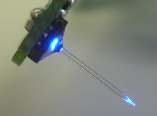
Figure: A High-Index Fiber Coated with Epoxy. The beads from as a result of surface tension and viscosity. Similar beads appear with MY133 adhesive, but not with the runny NO13685. This epoxy-coated fiber transports 30% of the light emitted by a blue EZ500 (480-μm square die).
The beading up of a coating on a fiber is incompatible with our ISL application. The photograph shows shows beads of epoxy on a length of our high-index fiber. The beads can be double the diameter of the fiber. The beads form in viscous adhesives whether we mount the fiber vertically or horizontally. Runny adhesives do not form beads, but they evaporate in the heat of the UV lamp before they cure.

We spilled our bottle of MY133, which will cost $400 to replace. Even if we can solve the problems of cleaning and curing these adhesives in a thin, uniform layer on our high-index fiber, we are not sure how we can apply a coating to an 8-mm fiber with a tapered tip. None of these adhesives can survive the temperature required to melt glass. We would have to coat the base of a 5-cm fiber, mount it in the stretcher, heat the glass to make the taper, then coat the glass up to the taper.

We conclude that the application of these coatings will be expensive, time-consuming, and unreliable. We will try to obtain cladded fiber with core refractive index 1.7 or greater. Such a fiber would provide us with sufficient numerical aperture on its own, and so greatly simplify the production of the ISL tapered fibers.

Discharge Rate and Capacity

We experiment with two types of lithium-ion battery. One is the PP031012AB, with nominal capacity 19 mA-hr. The other is the 382030 with nominal capacity 150 mA-hr. The small one we consider suitable for implantation in mice, and the larger for implantation in rats.

The data sheets give a maximum charging current of 9 mA and 80 mA for the small and large batteries respectively. We begin by charging the small battery at 20 mA and the large one at 150 mA until the battery voltages reach 4.3 V. We discharge both with resistors, and we find that the battery capacity is roughly half nominal.

We now charge the batteries by the rapid-charge procedure specified by their data sheets. We supply 9 mA to the small battery and 150 mA to the large battery until their voltages reach 4.3 V, then we apply constant voltage of 4.3 V until the battery current drops to 10% of the rapid charge current. After two hours, both batteries appear to be fully charge. We discharge them with resistors. The graph below shows the small battery discharging through a 200-Ω resistor (A) and the large battery discharging through a 40-Ω resistor (B).


Figure: Charging and Discharging Lithium-Ion batteries. Lines A and B showing the discharge of the small battery through 200 Ω and the large battery through 40 Ω. Lines C and D show the small and large battery charging up to 4.3 V. Lines E and F another discharge with the same resistors. Line G is the large battery discharging through 20 Ω, and H is discharging through 10 Ω.
At 3.7 V the discharge currents (A and B) are 18 mA and 92 mA respectively. While discharging to 3.0 V, the small battery delivers 20 mA-hr and the large one delivers 160 mA-hr. The small battery discharges completely to 0.0 V through the 200-Ω resistor. The large battery is equipped with a protection circuit that disconnects it from the 40-Ω resistor when the battery voltage drops below 3.0 V.

We recharge the large battery at 150 mA (C) and the small battery at 9 mA (D). We discharge through the same resistors (E and F). The large battery provides 162 mA-hr but the small battery provides only 11 mA-hr. The small battery has been damaged by its complete discharge to 0.0 v. We re-charge the large battery and discharge it through 20 Ω (G). At 3.7 V, the discharge current is 185 mA. The battery provides 148 mA-hr. We re-charge and discharge through 10 Ω (H). At 3.7 V, the discharge current is now 370 mA and the battery still provides us with 130 mA-hr.

Lithium-ion battery data denote the nominal capacity of a battery in mA-hr with the letter C. For our large battery, C = 150 mA-hr. The rapid charge current is 1.0C mA = 150 mA. The maximum discharge current is 160 mA, which is 1.1C mA. The smaller battery has C = 19 mA-hr, but its rapid charge current is only 0.5C, or 9 mA, and its maximum discharge current is also 0.5C.

It takes one or two hours to charge a lithium-ion battery to its nominal capacity 1.0C. When we discharge at 1.0C mA, the capacity drops to 0.9C mA-hr, and discharging at 2.0C mA, the capacity drops to 0.8C mA-hr. If we allow the battery to discharge completely to 0.0 V, it loses over half its capacity. Thus we can draw 38 mA continuously from our 19 mA-hr miniature lithium-ion battery and still obtain 15 mA-hr of battery life.

High-Index Fiber

We receive from Fiberoptics Technology several hundred meters of 0.016" clad rod, F2/8250. We measure its outer diameter as 390 μm. Its core is Schott F2 glass and its cladding is Schott 8250. The core occupies 83% of the fiber cross-sectional area. We have a 355-μm diameter core with a 17-μm layer of cladding. The rod is so thin we can bend it in a 10-cm radius, and the core has refractive index 1.63, so we will call it high-index optical fiber.

We take a 5-cm length of fiber and polish both ends. We try to use hot-glue to hold the fiber in a ferrule, which is our usual method with silica glass, but when we try to remove the hot glue with a propane flame, the glass melts. The F2 glass melts at only 434°C compared to 1100°C for the silica we usually work with. Our flame-based tapering machine will not taper this glass. We will have to develop a lower-temperature heater to take the fiber just above its glass temperature for tapering. We will have to devise a reliable method for polishing the flat end of the fiber without the use of hot glue. For now, we did the best we could holding it between finger and thumb.

We clean the fiber and coat it with NO13685 adhesive. This adhesive has the consistency and appearance of water when applied, and cures to a tacky solid in UV light. Its refractive index is 1.3685. We lower this fiber onto a green EZ500 LED. We pre-cure the coating, then add clear epoxy to hold the fiber in place, and cure further while blowing nitrogen over the exposed coating. (The coating cures to a non-tacky, flexible solid only in the absence of oxygen.) We turn on the LED and take a photograph of the fiber base with our microscope, shown below on the left.


Figure: High-Index Fiber with NO13865 Coating. Left: first attempt, note the epoxy holding the fiber onto the LED. Right: after cleaning the fiber with acetone and re-coating.

In the left-hand picture we see light escaping from the bottom of the fiber, from dirt beneath the coating, and from the meniscus of the epoxy where it encloses the fiber. The fiber tip emits 19% of the LED light (2.6 mW of green light from a total of 13.6 mW generated with 30-mA forward current). We wipe the fiber repeatedly with acetone. The coating comes off and we continue to clean the fiber until hardly any signs of dirt remain. We coat the fiber again, and cure the coating. We obtain the photograph on the right. The fiber tip now emits 24% of the LED light (3.2 mW). The signs of dirt on the coated fiber are greatly reduced, but we still see the same ring of light at the limit of the epoxy.

If we assume light is distributed uniformly across the 480-μ square area of the EZ500, then 43% of its light should enter our 355-μm fiber core and 9% should enter its cladding. The core of index 1.63, combined with the coating of index 1.3865, gives us a numerical aperture of 0.87, so we expect 76% of the light in the core to reach the tip. The cladding has index 1.487, and is combined with the same coating, so it has numerical aperture 0.58 and we expect 34% of the light in the cladding to reach the tip. Adding these up, we expect to get 36% of the LED light at the fiber tip. We see only 24%.


Figure: A 5-cm Coated Fiber on Green EZ500.

The photograph above shows that the light leaking from the exposed length of the fiber is small compared to the light emitted by the tip. Our close-ups of the base of the fiber, however, show a ring of light being lost from the fiber at the limit of the epoxy. It could be that the coating was improperly cured and the epoxy penetrated to the fiber glass along the epoxy meniscus. The epoxy has index 1.5, which reduces the numerical aperture of the cladding to 0.00 and the core to 0.61. A sufficiently lengthy contact between the epoxy and the glass would reduce the fraction of light reaching the tip from 36% to 16%.

Another potential loss of power at the tip is poor polishing of the fiber ends. In the past, we have observed 10% loss of power due to slight imperfections in the polish. The polish on the ends of this fiber is far from perfect.

Nevertheless, we are now seeing 24% of the LED light at the fiber tip, which is better than our previous record of 17%. When combined with our new and more efficient blue LEDs, this fiber would give us 7.2 mW at the fiber tip for a 30-mA LED current.

In the future, we will try the MY132 coating, with refractive index 1.325. This alone will increase our theoretical coupling efficiency from 36% to 42%. We may also find that the LED light is concentrated towards its center, as we did before, where a 300 μm fiber captured 9/5 as much light as we expected. Thus we might obtain up to 75% of the LED light at the tip.

UPDATE: [26-APR-13] Spoke to Adam at Norland Products and decided to try NO1625 and NO164 adhesives to glue the base of the fiber to the LED. These adhesives have refractive index 1.625 and 1.64 respectively, so they should fill scratches in the fiber base and give us a reliable optical connection between the silicon surface and the core glass.

UPDATE: [03-MAY-13] We achieve 30% capture efficiency with the F2-core fiber and a 460-nm EZ500. The LED emits 27 mW at 30 mA forward current and we see 8.2 mW at the far end of an 8-cm fiber coated with black epoxy. Only the 355-μm core carries light. Its numerical aperture with the cladding is 0.67. We expect 43% of the LED light to enter the fiber, and 45% of this light entering to reach the other end, for a total capture efficiency of 19%. With the fiber offset from the LED center, so as to avoid the cathode pad, we get 24%. But when we center the fiber, which requires that we smash down the cathode bond wire, we get 30%.

Lithium-Ion Batteries

The Implantable Lamp (A3024A) is powered by a BR1225 lithium primary cell. Its nominal voltage is 2.7 V and its nominal capacity is 48 mA-hr. It cannot be recharged, and we anticipate that its capacity when providing 10 mA will be closer to 24 mA-hr, because its nominal discharge current is only 30 μA. The A3024A provides 30 mA at 5.0 V for its lamp using a 90% efficient inductive boost regulator. But the battery's internal resistance is of order 40 Ω, and this resistance limits the continuous lamp current to 8.2 mA. The A3024A is equipped with a 1-mF capacitor bank in parallel with the battery, and this capacitor bank allows the boost regulator to flash the lamp for up to 10 ms. The volume of the capacitor bank is roughly the same as the volume of the battery. When we flash the lamp for 10-ms bursts every 100 ms, the battery voltage drops to 1.8 V as it provides an average current of 10 mA. We expect this current to exhaust the battery in 2.4 hrs.

The LIR1220 lithium-ion secondary cell is slightly thinner than the BR1225, has nominal output voltage 3.6 V, output resistance only 2 Ω, and can be re-charged. With its low output resistance, it can supply continuous power to the lamp without the need for a capacitor bank. Its capacity, however, is only 8 mA-hr. Consider instead the PP031012AB lithium-ion battery with capacity 19 mA-hr. Its rectangular shape occupies only 0.25 ml, compared to the 0.31 ml of the circular BR1225. When flashing the lamp 10 ms out of every 100 ms, the battery voltage will remain close to 3.6 V, and the battery will need to supply an average of only 5 mA to the boost regulator. The battery's capacity is 19 mA-hr at a discharge current of 20 mA. Here our average current is 5 mA but the peak current is 50 mA. We expect a slight decrease in capacity as a result, perhaps to 15 mA-hr. Even so, we can flash the lamp for 3.0 hrs with this battery, compared to 2.4 hrs with the BR1225. Furthermore, we can turn on the lamp continuously, although we should be aware that doing so will reduce our battery capacity.

The Implantable Sensor with Lamp (ISL), as we specified in our Technical Proposal, will combine a subcutaneous transmitter, an implantable lamp, and a microprocessor into one circuit that may be implanted in a rat. We are aiming to keep its volume less than 4 ml. Suppose we equip the ISL with a TE382030 battery pack. Its volume is 2.3 ml (30 mm × 20 mm × 3.8 mm), which leaves us 1.7 ml for the circuit, which will be sufficient because we no longer need space for a capacitor bank. The battery has capacity 150 mA-hr when delivering 150 mA continuously. It could flash the lamp with current 30 mA for 10 ms out of every 100 ms for 30 hrs, or it could turn the lamp on continuously for 3.0 hrs. Alternatively, with some lower-resistance lamp leads, we could increase the lamp current to 50 mA, thus boosting the optical power at the fiber tip, and we would still be able to turn on the lamp continuously for 1.8 hrs.

Lithium-ion batteries discharge themselves slowly. Even if we draw no current from them, they lose roughly 5% of their charge in the first month and 2% per month thereafter. This self-discharge, combined with their lower total capacity compared to the lithium primary cells, will shorten their shelf-life to a few months. If we could recharge the batteries before implantation, we could be sure of obtaining the maximum operating life after implantation. If we could recharge the battery while it is implanted, we could greatly extend the duration of our experiments.

The head fixture of the ISL offers us an opportunity to recharge a battery while implanted. Suppose we contrive to place upon the head fixture a sufficiently small, two-way, water-resistant socket. In addition to the L+ and L− leads required by the lamp, we run a B+ lead to the battery positive terminal on the ISL circuit. The B+ and L− wires connect to the two-way socket in the head fixture. When we want to recharge the battery, we connect two flexible leads with pins on the end to the head fixture. These leads in turn connect to an especially-designed battery charger, which we connect to our LWDAQ. The charger measures the resistance of the charging leads and monitors the battery voltage during a rapid charge cycle that will take roughly one hour to complete.

In both the mouse-sized Implantable Lamp and the rat-sized Implantable Sensor with Lamp, it appears that the lithium-ion battery pack provides us with a smaller, longer-lasting, and more capable power supply, even if we do not recharge them. Thus we believe we should switch to lithium-ion batteries for the ISL development regardless of whether or not we can devise a way to recharge the batteries while implanted. Furthermore, we will add a single pad to the ISL circuit that will allow connection to the battery positive terminal, so we can re-charge the battery before encapsulation, and allow for the possibility of recharging through a separate B+ lead to the head fixture.

UPDATE: [24-APR-13] We take an old cell-phone lithium-ion battery and solder wires to its terminals. This is a PBR-55D by Pantech, capacity 1000 mA-hr with nominal voltage 3.7 V. We use a 10 Ω power resistor as a load and a bench power supply as a charger. We have no difficulty charging and discharging the battery, and we find its output resistance to be 1.0 Ω. Further investigation reveals that the standard quick-charge time for lithium-ion batteries is 2.5 hrs. We begin with constant current charging at 0.5C/hr, where C is the battery capacity. When the battery voltage reaches 4.2 V, we switch to constant voltage charging until the charge rate drops to 0.05C/hr.

Cladded Rod

We receive from Tim Beeman of Fiberoptics Technology Inc. a sample of 1.2-mm diameter clad rod. The core of the rod is made of Schott glass type F2, with refractive index 1.63 for blue light and 1.61 for red. The cladding is Schott 8250 glass with index 1.49. We expect the numerical aperture of the rod to be 0.66 for blue light and 0.61 for red.

We cut a 200-mm length and cover it with black epoxy of refractive index 1.5 for half of its length. We polish both ends with diamond grit paper to give an optical finish. The epoxy makes sure no light gets into the rod through its curved surfaces. It mimics the epoxy we have been using to bind our fiber to our LED, and makes sure that the cladding of the rod is what causes total internal reflection in the core, rather than the cladding-air interface. We set up the cladded rod as shown below, with a 650-nm red laser beam shining into one end, and a screen to observe the pattern of light emitted by the far end. We place a black foam baffle around the near end of the rod.



The light entering the rod emerges in a cone, making a ring on our screen. When a light ray enters a cylindrical rod at an angle θ to the axis, reflections off the rod surface re-direct the ray, but do not change the angle it makes with the axis. When the ray emerges from the rod, after many reflections of a perfectly-cylindrical rod, it emerges at an angle θ to the axis. We see two cones for small angles of incidence, but in the photograph we are at 40° and the ring is clear and sharp. With a photodiode and our graduated screen, we measure the power emerging from the end of the rod and the angle of the cone it emits. We obtain the following graphs.



Our measurement of transmission becomes unreliable for angles bigger than 60° because the rod end presents such a small area to the laser beam. Nevertheless, we see that the rod captures and transports more than 50% of the light incident upon one end for angles 60° and lower. With numerical aperture 0.61, we expect to get total internal reflection within the rod for angles less than 38°. We see 80% transmission at 40° and 25% at 60°. We believe these results are consistent with numerical aperture 0.61.

If we could obtain such a rod with diameter 400 μm, its numerical aperture for blue light would be 0.66. With such a fiber we could capture 43% of light emitted by our LED and transport it to the fiber tip. If we coat this rod with a layer of adhesive with index 1.32, the coated rod will have numerical aperture 0.96. It will capture and transport almost all the light that enters its base from our LED.

UPDATE: [27-MAR-13] Fiberoptics Technology tells us they can make 400-μm clad rod of the same type studied here. We have ordered a batch to arrive in a few weeks. The company tells us that they believe they can make the same diameter clad rod out of glass with index 1.75. When combined with their cladding, a core of index 1.75 provides numerical aperture 0.92, with no need to use low refractive index adhesives.

UPDATE: [15-APR-13] We try out a Luxeon Z LED, the blue LXZ1-PB01 version. The LED emits roughly 29 mW for 30 mA forward current. The emitting surface of the LED is 1.2 mm square. We place our 1.2-mm diameter, 200-mm long clad rod over it and observe roughly 40% of the power emerging from the other end. The rod covers 80% of the emitting surface of the LED, so it appears that the rod is transporting 50% of the light that enters its base.

UPDATE: [16-APR-13] We receive several hundred meters of clad rod from Fiberoptics Technology. Its diameter is 390 μm. We can bend it with into a radius of 10 cm. We take a 20-cm length, polish both ends, and glue one end to our LXZ1-PB01 blue LED. We use UV-curing adhesive of refractive index 1.54. We coat most of the length of the rod in the same adhesive. We run 30 mA through the LED, so that it emits 29 mW. The rod covers 8.3% of the emitting area of the LED, so we expect 2.4 mW to enter the base of the rod. If the numerical aperture of the clad rod is 0.66, we expect 44% of the light to reach the other end, or 1.0 mW. We measure 1.4 mW at the other end. We press the rod tip against a piece of white paper so we can see the cone of light it emits. The angle at the base of the cone is roughly 74°, which suggests a numerical aperture of 0.60.

Fiber-Cladding Adhesive

When we make a Head Fixtures (A3024HF), there is a stage at which we have the 7-mm long, tapered fiber positioned above the bare LED, ready to be glued in place with clear epoxy. At this step, we can apply current to the LED if we like, and observe light leaking out of the base of the fiber and shining out of its tapered tip.

We applied 30 mA to a blue EZ290 LED and held a 10 mm × 10 mm photodiode 5 mm above fiber tip. We obtained a photocurrent of 1.2 mA, which corresponds to 6.0 mW of blue light. This seemed odd to us, so we repeated the measurement several times. This particular LED was emitting 18 mW at 30 mA, and our calculations based upon the fiber's numerical aperture suggested that no more than 3 mW should be emerging in total from the fiber tip.

We applied clear epoxy (E30CL) to the fiber base, with power still applied to the LED. The intensity of the light emitted by the tip of the taper decreased immediately, while that of the light emitted from the base of the fiber increased. We measured once again the power 5 mm from the tip of the fiber. We observed only 1.5 mW. Later, we measured power emitted in all directions with the same fiber tip and obtained a total of close to 3 mW.

The numerical aperture of an optical fiber is the greatest angle a ray entering a polished, perpendicular face can make with the fiber axis and still be constrained within the fiber by total internal reflection. This total internal reflection can occur at the core-cladding boundary, which is always available, or at the cladding-glue boundary, or the cladding-air boundary. The following calculation shows how the numerical aperture of the fiber is affected by glue and air.



The WF300/330/P37 fiber has a cladding of fused silica, with refractive index n₃ = 1.458. Its specified numerical aperture is 0.37, which is the numerical aperture we get by total internal reflection at the core-cladding interface. The refractive index of the air outside the base of the fiber is n₁ = 1.000. Using the equation derived above, we conclude that the germanium-doped core of the fiber has refractive index n₂ = 1.504. Now suppose we surround the fiber with clear epoxy. Our clear epoxy has refractive index n₄ = 1.5. Because the glue has higher refractive index than the cladding, there will be no internal reflection at the cladding-glue boundary.

When we are assembling a head fixture, we hold the fiber in a clamp that touches the cladding along three contact lines each 5 mm long, so the majority of the cladding surface is exposed to air. Under these conditions, our equation gives us a numerical aperture of 1.1, which we interpret to mean that any ray entering the fiber will be trapped by internal reflection at the cladding-air boundary. Thus we expect to see all the power entering the base of the fiber emerging at the tip. Our fibers were not perfectly clean, so we were losing some light because of oil on the cladding surface, but we do see four times as much power when we hold the fiber without glue in a clamp.

Suppose we use a glue with a lower refractive index than the cladding. We will now see total internal reflection at the cladding-glue interface. Consider the MY132, UV-curing adhesive, designed specifically for cladding optical fibers. It is expensive (roughly $300 for 10 ml). But its refractive index is only 1.324. With this adhesive fastening the fiber to our LED, and coating the fiber up to the base of the taper, the numerical aperture of the fiber would be increased to 0.71, which means that light within a ±46° cone will be accepted and constrained within the fiber.

With numerical aperture 0.37, we expect to capture 14% of the light emitted by an EZ500 LED. This calculation is borne out by our measurements. But with numerical aperture 0.71 we will capture 51% of the emitted light. The power delivered to our fiber tip will increase by almost a factor of four.

We have learned from Cree that their EZ290 LED will not produce the optical power we expected. The most efficient LED we can buy is the EZ500. We believe the most efficient class of these LEDs will emit 30 mW of blue light with forward current 30 mA. A well-positioned 400-μm diameter fiber covers 90% of the light-emitting surface of the EZ500. Thus we can hope for 27 mW to enter our adhesive-coated fiber, and 14 mW to emerge from the tip. We plan to order a reel of the most efficient class of EZ500 LEDs, and a sample of the MY131MC adhesive, and test our hypothesis.

Another way to increase the numerical aperture of the fiber is to increase the refractive index of its core. We have ordered a sample of 1.4-mm diameter borosilicate glass rod from Fiberoptix, which has refractive index 1.6. We will try to stretch this to create a fiber of diameter 400 μm which, when coated by MY132, will provide numerical aperture 0.90 and therefore capture 81% of the LED light. We would then be able to deliver 22 mW to the fiber tip.

Stage Three Delivery

Today we ship to ION the following components:

• 5 of Head Fixture (A3024HF)
• 1 of Implantable Lamp (A3024A)
• 2 of White Test Lamps
• 1 of Command Transmitter (A3023CT)
• 1 of Booster Amplifier (ZHL-3A)
• 1 of 24-V Power Supply for Booster Amplifier
• 1 of Flexible Antenna with 2-dB Attenuator
• 1 of Telescoping Antenna with BNC elbow
• 1 of Coaxial Cable with 12-dB Attenuator

Early next week we plan to ship the following, which will complete the deliveries required by ISL Stage Three, Design and Construction of the Implantable Lamp.

• 4 of Implantable Lamp (A3024A)

In the photograph below, we see the Command Transmitter (A3023CT) connected directly to the Flexible Antenna. The 2-dB attenuator at the base is necessary to stabilize the A3023CT's power amplifier. This arrangement supplies 100 mW of 146-MHz RF power to the antenna, and is easy to set up. We use this arrangement for test that do not require us to operate more than 50 cm from the antenna. We determine the length, number, and spacing of RF power pulses using the same control program that we use with the Lamp Controller (A2060L).



The same photograph shows one Implantable Lamp (A3024A) flashing a white LED, and another at with a paper insulator around its L+ lead. The paper insulation is needed to stop the A3024A contact pins from touching when stored in a bag. If they touch and the lamp is stimulated, we will waste battery capacity supplying current to the lead resistance. The white LED is one of our White Test Lamps, which we have equipped with sockets to accept the pins on the tips of the A3024A leads. The test lamp leads have color codes and socket orientation to mimic the head fixtures and the colors of the A3024A leads.



When we want to operate farther from the antenna, and allow for random movements of the receiver, we add a ZHL-3A booster amplifier between the A3023CT and the antenna, and we use a telescoping antenna instead of the shorter flexible antenna. The telescoping antenna is more efficient. In this arrangement, we must be sure to insert the 12-dB attenuator between the A3023CT and the ZHL-3A, so as to protect the ZHL-3A's input from over-drive. With this arrangement, we obtain 100% reliable stimulation of the implantable lamps at range 1 m in our basement laboratory and 2 m in a faraday tent. This operating range is double that which we set as our target.



The telescoping antenna, being 1 m tall, needs to be vertical or else it will fall over. The ZHL-3A amplifier gets warm after a few minutes. We have found it to be rugged, but the manufacturer recommends that you connect its load (the antenna) and input (the cable carrying 146 MHz) before you connect power (the 24 V supply) in order to protect it from over-drive.

The Head Fixtures (A3024HF) are equipped with sockets for the A3024A contact pins. They are equipped with dummy cannulas in their guide cannulas. We have applied black epoxy over the clear epoxy that holds the fiber to the LED and the circuit board to the guide cannula. The black epoxy serves to mask light that escapes through the base of the fiber, which is roughly 85% of the light emitted by the LED. By masking this light, we are better able to estimate the power emitted by the fiber tip, and we avoid flashing a bright light into the subject animal's field of view, which might otherwise corrupt our experiment. The disadvantage of our black covering of epoxy is that the experimenter may not be able to confirm by inspection whether or not the implantable lamp is responding to commands. In future designs, we will consider placing a separate LED on the back of the head fixture to emit a small amount of light as an indicator for the experimenter.



It is hard to measure the total power emitted in all directions by the fiber tapers. Nevertheless, we tried to do so and obtained 2.5±1 mW. When we tested the fibers before we tapered them, we obtained 3±0.2 mW. These results are consistent, and suggest that the total power is a little below 3 mW. This 3 mW is well below our target of 10 mW. In the future, we will increase the power output at the tip by using a higher numerical aperture fiber, or higher drive current, or a more efficient LED, or some combination of all three modifications.

Prototype Head Fixture

The following photograph shows our first assembled fiber and cannula Head Fixture, following the design we presented earlier. The small ruler graduations are 0.5-mm. The fiber diameter is 300 μm.



Part (4) is the fiber, one end of which is glued with clear optical epoxy to an EZ500 LED mounted on the circuit board. This fiber is a dummy we used to make a prototype head fixture. Its tip is sheared off at an angle instead of tapered with a flame.

Part (1) is the L+ lead from an Implantable Lamp (A3024A). Part (2) is the connector pin on the end of the L− lead from the same device. These pins plug into two sockets on the Head Fixture. Part (3) is the L− socket. The L+ socket is obscured by L−. Part (8) is the head fixture circuit board. Part (5) is a silica guide cannula. Part (6) is the threaded pedestal on the guide cannula. Part (7) is a smoothing capacitor to reduce noise induced in EEG recordings.

Measured Capture Efficiency

We have four different types of optical fiber and two different types of light-emitting diode. We make three samples of each fiber, which we name 1 to 3 for each type. Each fiber has two faces, A and B. We lower each face of each fiber onto an LED in turn and measure the power emerging from the other face.



Figure: Fraction of Power Captured By Fibers. The 480-μ square LED is the C460EZ500. The 290-μm square LED is the C470EZ290.

In the above table, we calculate the theoretical capture fraction in two steps. First, we estimate the fraction of light that will enter the fiber, based upon the area of the fiber and the area of the LED. Second, we apply our cosine-distribution solution to the capture efficiency of a fiber of known numerical aperture, which we present here.

In the case of the 400-μm fiber over the 290-μm square LED, we assume all the LED's light enters the fiber. The fiber is larger than the diagonal of the square, and placed within 50 μm of the LED surface by pressing down the bond wire. We observe 15% capture fraction and calculate 14%. Our calculation based upon the fiber numerical aperture appears to be accurate.

In the case of the 300-μm fiber over the 480-μm LED, we assume that only 30% of the light will enter the fiber. But our observed capture fraction is 9% and our calculation is 5%. Given that we already trust our numerical aperture calculation, we suspect that twice as much light is entering the fiber as we expected, which in turn means that the light emitted by the 480-μm square LED is concentrated towards the center.

When we place a 400-μm fiber with NA = 0.37, NA = 0.25, or NA = 0.24 on the 480-μm square LED, the capture fraction we measure is roughly 1.6 times the one we calculate. This result is also consistent with concentration of light towards the center of the light-emitting area.

Our 300-μ NA = 0.41 fiber's capture fraction with the 290-μm LED is 17%. With a 400-μm, NA = 0.37 fiber on the same LED we get 15%. If we assume that all the light from the LED enters both fibers, then the difference in capture fraction is consistent with our calculation due to numerical aperture. This suggests that the light emitted by the 290-μm LED is also concentrated towards the center, so that all of the light enters the 300-μm fiber.

We conclude that our numerical aperture calculation, which assumes a cosine distribution of light emission by the LED, is accurate, but our assumption of uniform distribution of light across the LED is not. The light is concentrated towards the center of the emitting area. Thus we are able to obtain almost double the capture fraction that we would with uniform light distribution.

With the 300-μm, NA = 0.41 fiber on the EZ290 we get 17% of the light emitted by the LED emerging from the tip of our fiber. If we could obtain a C470EZ290 that emitted 40 mW for 30 mA current, as specified by the data sheet, we would obtain 6.8 mW at the fiber tip. As it is, our EZ290s are producing only 17 mW at 30 mA, so we see only 3.0 mW. We do not know why our EZ290s are performing so poorly. The are emitting less than half the light we expect from the calibration sheet supplied with our samples. It may be that they have aged from exposure to air over the past year and a half since we received them. In the case of the EZ500, the LEDs produce 25 mW for 30 mA current, and we get 11% capture efficiency with our 400μm, NA = 0.37 fiber. So we obtain 2.6 mW at the fiber tip.

As things stand today, we can obtain roughly 3 mW with both the EZ290 and the EZ500, using our high numerical aperture 300-μm and 400-μm fibers respectively.

LED Efficiency

We measure the total power emitted by a selection of LEDs. To measure optical power we use an SD445 photodiode. It's sensitivity to light of various wavelengths, in Ampere per Watt, is given in the figure below. We press the photodiode right up against the package of our LED, so that is roughly 2 mm from the light-emitting surface.



We reverse-biase the photodiode with a 9-V battery and pass the photocurrent through a 100-Ω resistor. We measure the voltage across the 100-Ω resistor with a voltmeter. We convert photocurrent into optical power using the graph above. At 470 nm we use 0.20 A/W. At 527 nm we use 0.25 A/W. We provide power to the LED through a 400-Ω, 1-W resistor. We measure the LED current with an ammeter. We obtain the following plots of output power versus current.



According to the EZ290 data sheet, the minimum power output of the blue C470EZ290-021 at 20 mA forward current should be 21 mA. According to the calibration of our sample diodes, the power should be at least 27 mW for this particular LED. But we measure only 13 mW. According to the same data sheet and calibration, the green EZ290s should produce at least 11 mW at 20 mA. But we measure only 6 mW. The EZ500 data sheet, meanwhile, specifies a minimum of 40 mW of green light at forward current 150 mA. We see 26 mW at 46 mA, which suggesets of order 85 mW at 150 mA.

Our green EZ500 emits twice as much power as we expect, but our blue and green EZ290s appear to be emitting less than half the power we expected from their calibration and specification. The blue EZ290 shown above will emit only 18 mW with a forward current of 30 mA, such as we expect to deliver with our Implantable Lamp (A2024A). Even if we obtain 25% coupling efficiency into our fiber, we will get no more than 4.5 mW out of the fiber tip.

UPDATE: [26-APR-13] We have 25 C460EZ500 (460 nm blue) mounted in 3-mm packages. We measure the light power emitted by one such part with a photodiode. We bias the photodiode with 0 V and with 9 V. The photocurrent is 6% higher with bias. The responsivity of the un-biased photodiode is roughly to 0.182 for 460-nm light and 0.191 mA/mW at 470 nm.

UPDATE: [22-JAN-14] The surface of the SD445 appears to be acrylic glass, which has reflectance with angle of incidence in air as plotted below. We obtained this and the following plot from Refractive Index Info.



The silicon of the photodiode we assume to be crystalline, which has the following reflectance with angle of incidence in air. By reflection alone, we expect to lose around 44% of incident unpolarized blue light by reflection at the acrylic and silicon boundaries for light arriving perpendicular to the surface. We calculate the sensitivity of the ideal photodiode, where one photon becomes one electron, is 0.38 mA/mW for 470 nm. If we lose 44% of incoming photons by reflection, we expect our SD445 to have sensitivity 0.21 mA/mW. The data sheet says 0.20 mA/mW.



At larger angles of incidence, we will lose more light by reflection, so the sensitivity of the photodiode will drop. At 80° we expect to lose around 60% by reflection, compared to 40% at 0°, so sensitivity will drop to 0.13 mA/mW.